

- Description
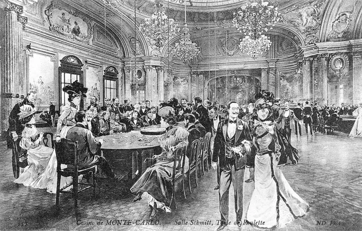
- A roulette table at the Monte Carlo casino
- Source
- Neurdein Frères · original page
- Licence
- PD Public domain
 The representativeness heuristic
“It looks like” becomes “it probably is”: resemblance takes the place of statistics.
In brief
- What: we judge that a case belongs to a category because it resembles our mental image of it, without taking into account how many cases there are in each category.
- Why: judging resemblance is easy and immediate; computing a probability is slow and costly. The brain substitutes the former for the latter.
- Detect: “he fits the profile perfectly” or “this project is just like the last one” without anyone citing a rate or a sample size.
- Avoid: start from the base rate (how many cases of each kind exist), adjust for the clues only afterward, and beware of small samples.
Definition#
 Fictitious illustration
 Illustration inspired by the person
The representativeness heuristic is a judgment shortcut described by Amos Tversky and Daniel Kahneman in the early 1970s: to decide whether an object A belongs to a class B, or whether a sample comes from a given process, we look at how much A resembles the typical idea of B. The stronger the resemblance, the higher the estimated probability.
The shortcut is often useful: what looks like a duck is, most of the time, a duck. It becomes a bias when resemblance says nothing (or almost nothing) about probability: ignoring the base rate, judging a small sample as if it reflected the whole, expecting a random sequence to “look” random, failing to see that a more detailed story is less probable than a shorter one.
The mechanism#
The bias rests on attribute substitution: to the hard question (“what is the probability?”) the brain answers an easy question (“does it look like it?”), without noticing. Four typical errors follow:
- Base-rate neglect: we forget that, in the population, the category is rare or common.
- Insensitivity to sample size: five cases “are enough” to identify a trend, although they vary a lot by chance.
- Conjunction fallacy: a rich, coherent description seems more probable than a simpler description that contains it.
- Misconceptions of chance: after a long run of “heads,” we expect “tails” (the gambler's fallacy), because a balanced sequence looks more like what we picture as randomness.
Kahneman and Tversky (1973) show participants short descriptions of people, supposedly drawn from a group of 100 engineers and lawyers. In one case, the group has 70 engineers and 30 lawyers; in the other, 30 engineers and 70 lawyers. Participants judge the probability of being an engineer almost the same way in both cases: they rely on how closely the description resembles a typical engineer, and ignore that the composition of the group completely changes the starting probability. When given no description, they use the proportions correctly; it is the presence of a detail, even a worthless one, that leads them astray.
Tversky and Kahneman (1983) describe Linda, 31, single, outspoken, very bright, a philosophy graduate, concerned with issues of discrimination and social justice. They then ask which statement is more probable: (1) Linda is a bank teller; (2) Linda is a bank teller and is active in the feminist movement. About 85% of participants (students with no training in statistics) judge the second more probable. This is logically impossible: the set of feminist bank tellers is included in the set of bank tellers. The description “resembles” a feminist more, and this criterion wins out over the logic of sets.
The Linda problem (1983)
Loading the chart…
View the data
| Wrong answer | Correct answer | |
|---|---|---|
| “Bank teller and feminist” judged more probable | 85 | - |
| “Bank teller” judged more probable | - | 15 |
Where you encounter it#
In project management#
- Analogy-based estimating: “it's like last year's project”; we hold on to the surface resemblance (same technology, same client) and forget to check how many “similar” projects actually met their deadlines.
- Bug diagnosis: “it looks like the bug from last time, it's surely the same cause”; we look where we have already found something, without checking the frequency of the possible causes.
- Proof of concept or pilot: two or three enthusiastic users (small sample) are taken to be representative of all users.
- Choice of a supplier: “they have the same culture as us, they look serious”; the sales team's profile stands in for the probability of good delivery.
- Reading indicators: three weeks without an incident are seen as a trend, or two incidents in a row as a “black streak,” although chance produces such sequences.
In management#
- Recruitment and promotion: we look for “the typical profile of a good developer” or “of a good project manager”; a candidate who resembles it is judged more likely to be good, with no regard for the actual success rate of profiles of this type (see similarity bias).
- Talent spotting: “he speaks well in committee, he's a future manager”; speaking ease resembles leadership, without measuring its probability.
- Evaluating a team: one month of good results is enough to label a team “high-performing,” although the sample is too small to tell talent from chance.
- Career narrative: a detailed, coherent background (“formerly at such-and-such company, passionate, results-oriented”) seems more probable than a plain one, although each added detail reduces its probability (conjunction fallacy).
Famous cases#
The 26 blacks at the Monte Carlo casino August 18, 1913#
Biases involved: misconceptions of chance (gambler's fallacy), representativeness.
What happened. On the night of August 18, 1913, at the Monte Carlo casino, the ball landed on black twenty-six times in a row at a roulette table. According to the classic account, players bet more and more on red, convinced that a long run of blacks had to be “compensated,” and many lost very large sums (millions of francs are mentioned; the exact figure varies from one account to another). The roulette wheel has no memory: on each spin, the probability of each color was the same as on the previous one.
What this illustrates
A run of twenty-six blacks does not look like what we expect from chance, hence the impression that it must be corrected. It is resemblance speaking, not probability. In a project, the same error is heard in: “we've had five failed deployments in a row, the next one will be fine” or, conversely, “we've had three good sprints, velocity is stable.” A short run says little; what matters is the process that produces it.
Linda, the textbook case of the conjunction fallacy 1983#
Biases involved: representativeness, conjunction fallacy.
What happened. In Tversky and Kahneman's (1983) direct test, participants rank eight statements about Linda by probability. The vast majority place “bank teller and feminist” ahead of “bank teller.” The error persists, somewhat attenuated, among more sophisticated participants, including doctoral students trained in probability. By contrast, when the question is asked in terms of frequencies (“out of 100 people like Linda, how many are bank tellers? how many are bank tellers and feminists?”), the error drops markedly: this finding is the basis for the countermeasures in the next section.
What this illustrates
The most detailed and coherent story is seductive, but every added detail makes it less probable. In a risk review or an incident scenario, a precise account (“the outage comes from the network update triggered by the contractor during the cutover”) seems more credible than a general cause (“a network outage”), although it is less so.
Warning signs#
- “He fits the profile perfectly” or “smells like the same problem as last time,” with no rate or proportion cited.
- A conclusion drawn from three, four or five cases (users, deployments, candidates, sprints).
- The description of a case is longer and more colorful than the figures that accompany it.
- Nobody asks “how many of each kind are there, in total?”.
- A run (good or bad) is read as a sign of “return to normal” or of a “trend” without analysis.
Avoidance reflexes#
- Ask for the base rate. Before any judgment: “of cases of this type, what proportion go like this?” An estimate by reference class (comparable projects, not just the one project that looks alike) is the best antidote.
- Start from the base, then adjust. Write down the starting probability (for example 30% of projects of this kind overrun their deadline by more than 30%), then adjust according to the real strength of the clues; resemblance alone is a weak one.
- Look at the sample size. “How many cases is this impression based on?” Three cases do not make a rule.
- Think in natural frequencies. “Out of 100 projects, how many…” speaks to intuition better than “30% probability.”
- Check for inclusion. When a scenario seems more probable because it is more precise, compare it with the simpler version that contains it: it cannot exceed it.
- Distinguish resemblance from prediction. For a hire, replace “does he resemble the good ones?” with criteria tied to success in the role (work-sample tests, verified references), applied the same way to all candidates.
- Remember that chance produces runs. Before interpreting a sequence of events as a trend, ask whether a sequence of that length would be surprising by pure chance.
With AI: detect, remedy, mitigate#
AI can recall the base rate, do the probability calculation and ask the questions we forget. But language models themselves reproduce conjunction and representativeness errors, and they readily produce plausible but made-up “statistics”: ask them for methods and sources, and check the figures.
Detect#
- Spot resemblance-based judgments (“typical profile,” “same cause as…”) in a recruitment file, a report or an incident analysis.
- Flag conclusions drawn from a tiny sample.
- Pick out overly detailed scenarios presented as the most probable.
Fix#
- Find the relevant reference classes and list the data to collect for the base rate.
- Do the Bayesian calculation of a probability step by step, with your figures.
- Restate a probability in natural frequencies (“out of 100 cases…”).
Mitigate#
- Generate selection criteria tied to the role, independent of resemblance.
- Have it propose competing explanations for an incident, with their relative plausibility.
- Produce a dashboard that separates runs (chance possible) from trends (lasting deviation).
Prompts to build into your routines#
1. Base rate before judging. When you are tempted to conclude “it looks like…”.
I am tempted to conclude that [case] is of type [category] because [resemblance elements].
Before answering me:
1. Tell me what base rate I would need to know to estimate this probability, and where I could find it (without making up a figure).
2. Explain how the resemblance elements I cite are weak or strong clues.
3. Propose a three-step method for combining the base rate and these clues.
If you do not know a figure, say so instead of estimating it.
2. Sample and chance check. When a conclusion rests on a few cases or on a run.
Here is what I observe: [description of the cases or the run, with their number].
Tell me: 1) what these observations reasonably allow me to conclude and what they do not; 2) whether chance alone could produce a run of this kind; 3) what additional data would be needed to tell a trend from a fluctuation; 4) a cautious wording of the conclusion I can communicate.
3. Competing scenarios. For an incident analysis or a risk review.
Here is the scenario we judge most probable: [detailed scenario].
Break it down into its elementary assumptions. For each, estimate its plausibility qualitatively, then say whether the complete scenario can be more probable than its simplified version. Propose three less detailed competing scenarios and say which checks would allow us to tell them apart.
How to build them in#
- Estimating and risk review: prompt 1 serves as the first question whenever an analogy is invoked.
- Incident review: prompt 3 forces you to write scenarios less detailed than the one you prefer.
- Steering: prompt 2 is useful before presenting a trend to a committee.
Precautions#
- An AI that gives you a base rate “from memory” may be wrong or make it up: demand the source and check it.
- Models themselves tend to judge the most detailed description more probable: do not delegate the decision to them.
- Do not paste candidate files or named evaluations into an unauthorized tool; anonymize.
- An AI used to screen candidates reproduces the resemblances present in its data: that is a risk in itself.
Limits#
- Representativeness is not always an error: when resemblance is correlated with the real probability, the heuristic gives good results at low cost. The bias begins when it replaces base rates.
- The interpretation of the Linda problem has been debated (the meaning of the word “probable,” the wording of the question); results vary with the presentation, and the frequency format reduces the error (Gigerenzer and Hoffrage, 1995). The phenomenon itself remains solidly replicated.
- The Monte Carlo story is a classic cited at second hand; the date and the 26 spins are consistent, the amounts lost much less so.
Sources and verification#
- Tversky & Kahneman (1974), “Judgment under Uncertainty: Heuristics and Biases,” Science — representativeness, base rate, sample size.
- Kahneman & Tversky (1973), “On the psychology of prediction,” Psychological Review — the engineers and lawyers problem.
- Tversky & Kahneman (1983), “Extensional versus intuitive reasoning: The conjunction fallacy in probability judgment,” Psychological Review — the Linda problem.
- Kahneman & Tversky (1972), “Subjective probability: A judgment of representativeness,” Cognitive Psychology.
- Gigerenzer & Hoffrage (1995), “How to improve Bayesian reasoning without instruction: Frequency formats,” Psychological Review — natural frequencies.
- Wikipedia (English), “Gambler's fallacy” — the Monte Carlo episode (1913).
- Kahneman, D. (2011), Thinking, Fast and Slow, Farrar, Straus and Giroux.
See also#
Counterweights and related reflexes#
What neutralises it.
- Reference class forecasting
- Le raisonnement sur les fréquences naturelles (concept or method, no page)
